ggplot2 is a data visualization package widely used for creating sophisticated plots. It was developped by Hadley Wickham and is based on the Grammar of Graphics (gg), which is a systematic framework for understanding and constructing data visualizations.
To get started !
Ensure tidyverse is installed
The ggplot2 package is part of the tidyverse (Hadleyverse).
First, ensure tidyverse is installed : install.packages('tidyverse')
library("tidyverse") #Load the library
── Attaching core tidyverse packages ──────────────────────── tidyverse 2.0.0 ──
✔ dplyr     1.1.3     ✔ readr     2.1.4
✔ forcats   1.0.0     ✔ stringr   1.5.0
✔ ggplot2   3.4.3     ✔ tibble    3.2.1
✔ lubridate 1.9.2     ✔ tidyr     1.3.0
✔ purrr     1.0.2
── Conflicts ────────────────────────────────────────── tidyverse_conflicts() ──
✖ dplyr::filter() masks stats::filter()
✖ dplyr::lag()    masks stats::lag()
ℹ Use the conflicted package (<http://conflicted.r-lib.org/>) to force all conflicts to become errors
The storms database
As in the dplyr tutorial, we will work with the storms dataset to present the package. Thanks to the tidyverse library, we have already loaded the dplyr package. storms is the NOAA Atlantic hurricane database best track data. The data includes the positions and attributes of storms from 1975-2021. Storms from 1979 onward are measured every six hours during the lifetime of the storms.
If you want to learn more about storms :
?storms
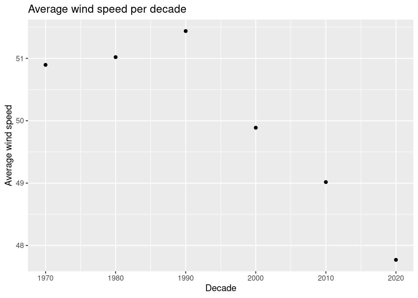
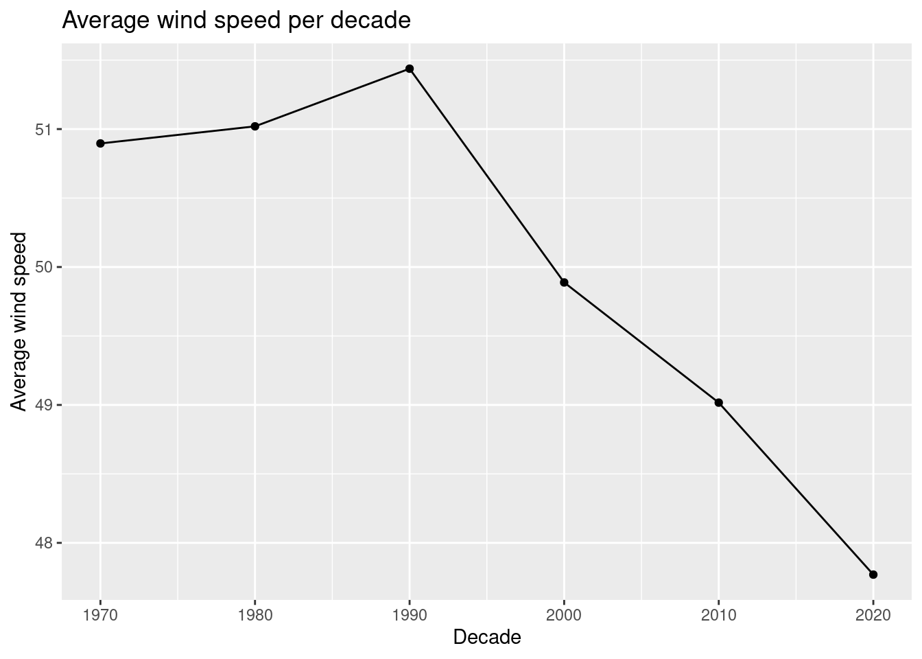
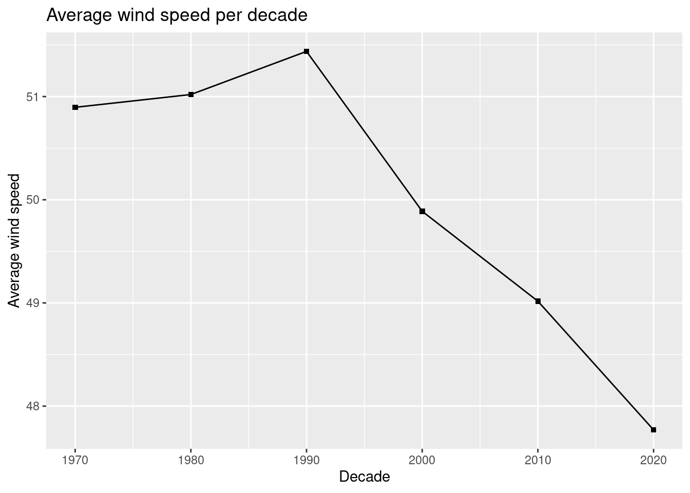
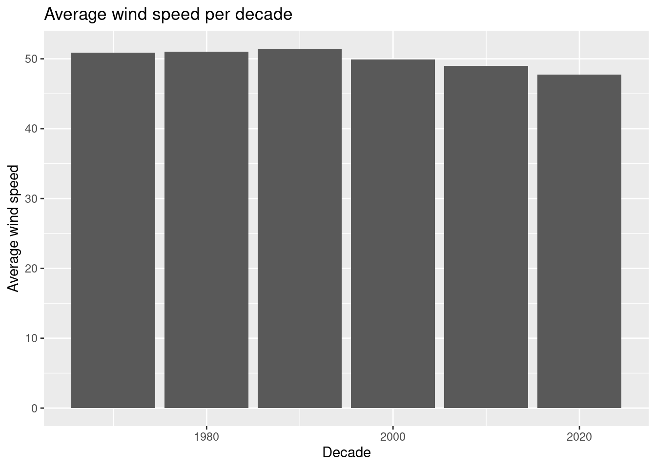
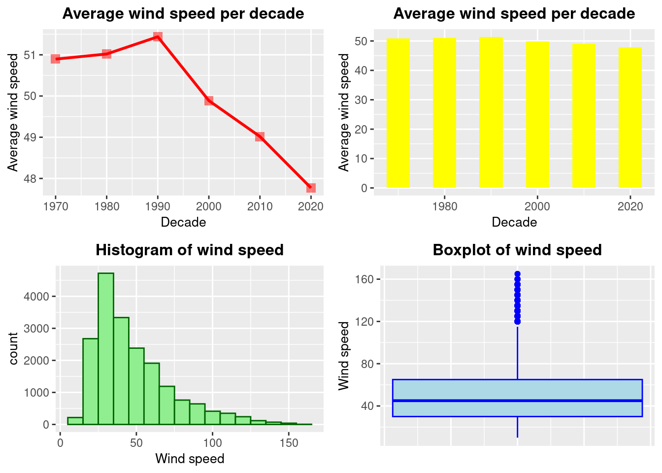
For example, we will be looking at the average, minimum and maximum wind speed of storms per decade. To do this, we create the storms_decade dataset :
To create a plot, the key elements to be specified are:
the dataset
the mapping of variables to aesthetics (like x and y axes, color, shape, size, etc.)
the geometric objects that represent the data (e.g., points, lines, bars, etc.)
ggplot()
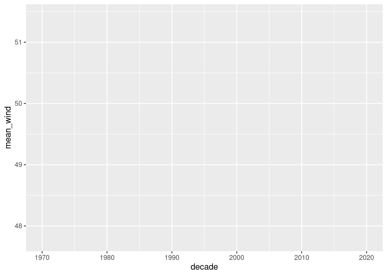
To initialize a plot, the key function of the package is ggplot(). The first argument data represents the data frame containing the variables to be plotted. Then, the aes() argument maps variables to aesthetics (e.g. x-axis, y-axis, color, size, etc ). Finally, layers from geometric object functions (e.g. geom_point, geom_line, geom_bar) allow to visualize data.
The ggplot() function doesn’t plot anything—it sets up the plot.
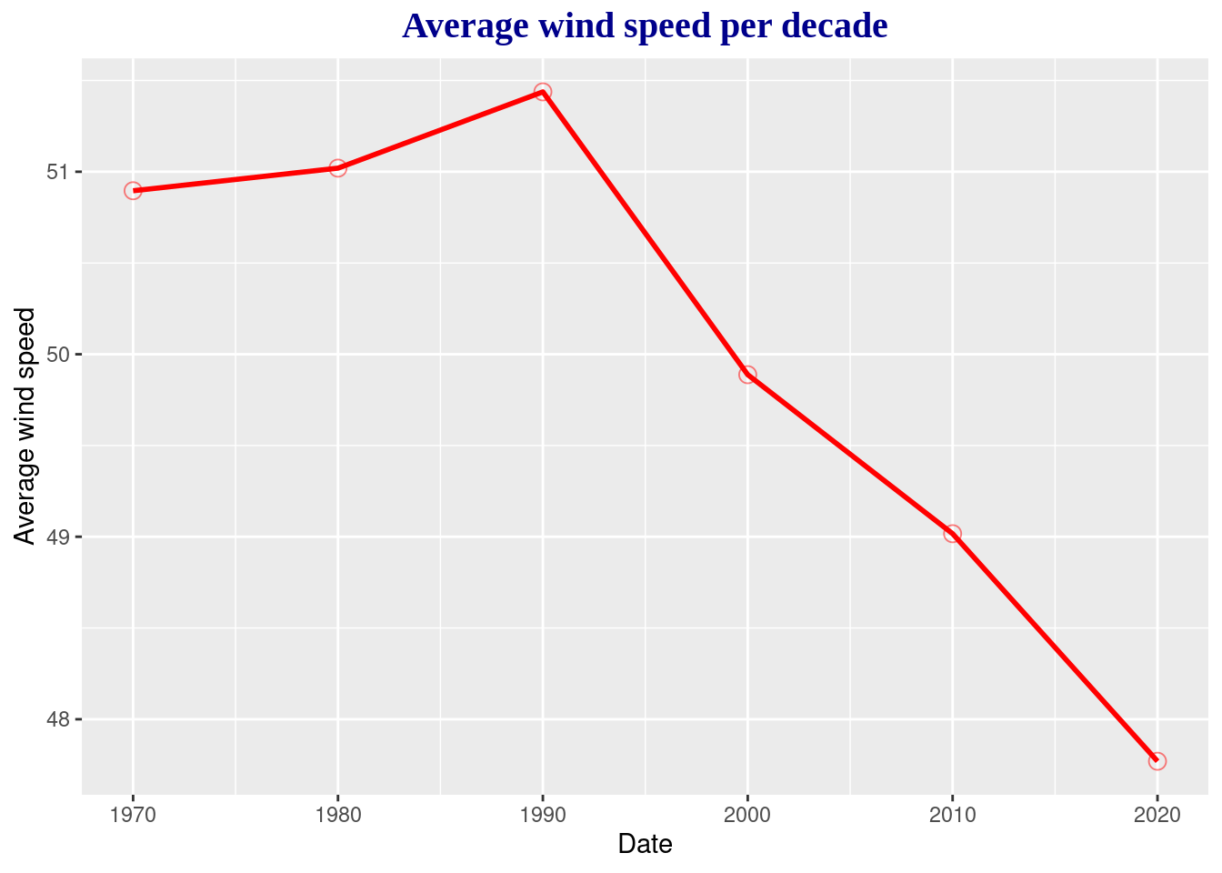
ggplot(data = storms_decade, aes(x = decade, y =mean_wind))
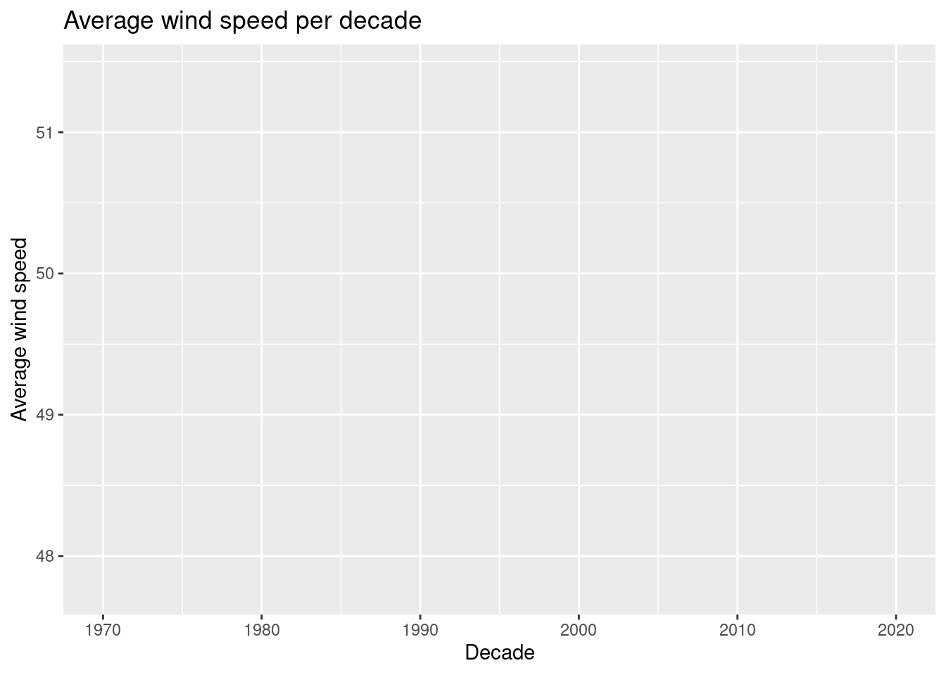
You can choose the titles of the plot as well as the x-axis and the y-axis with labs:
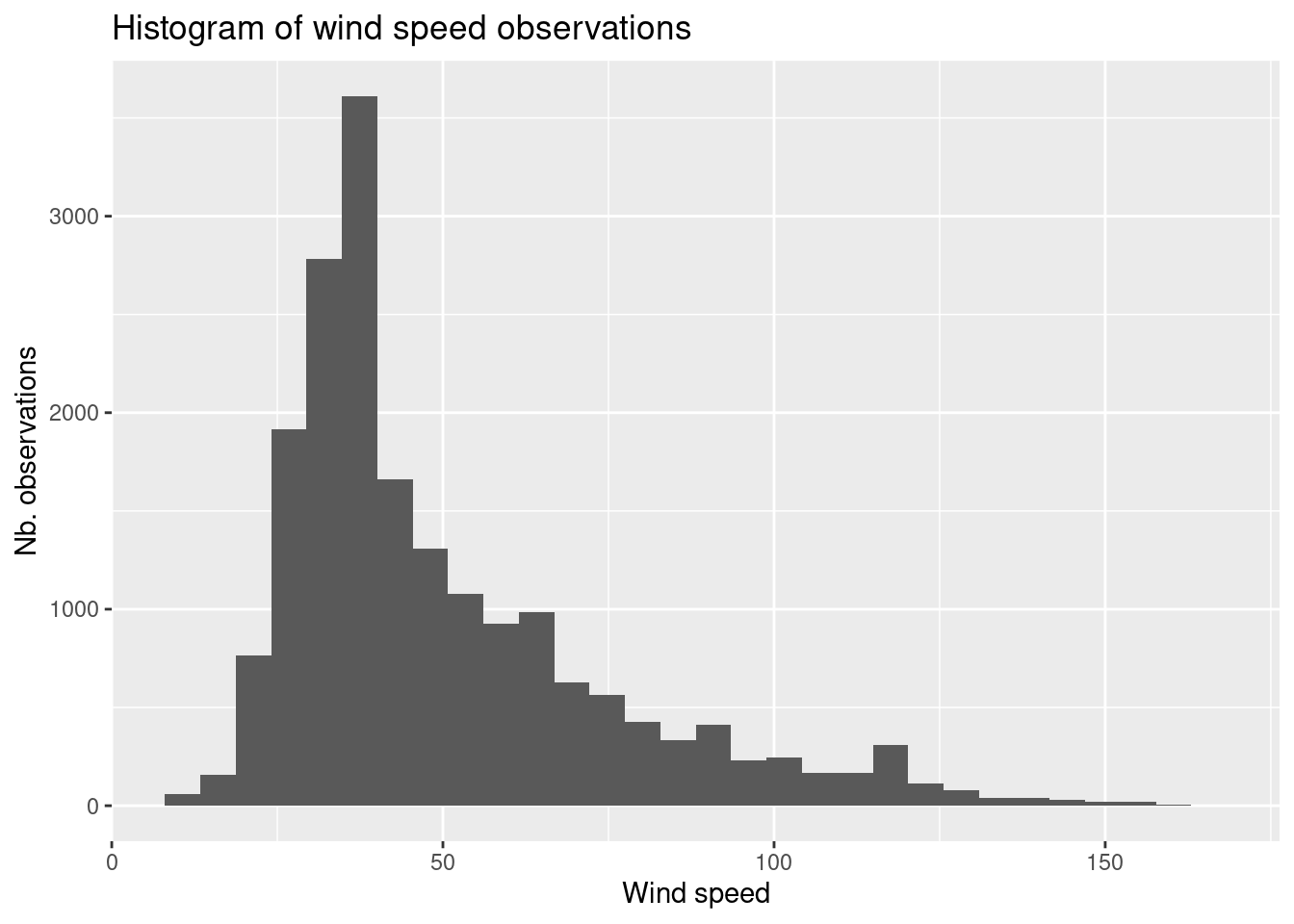
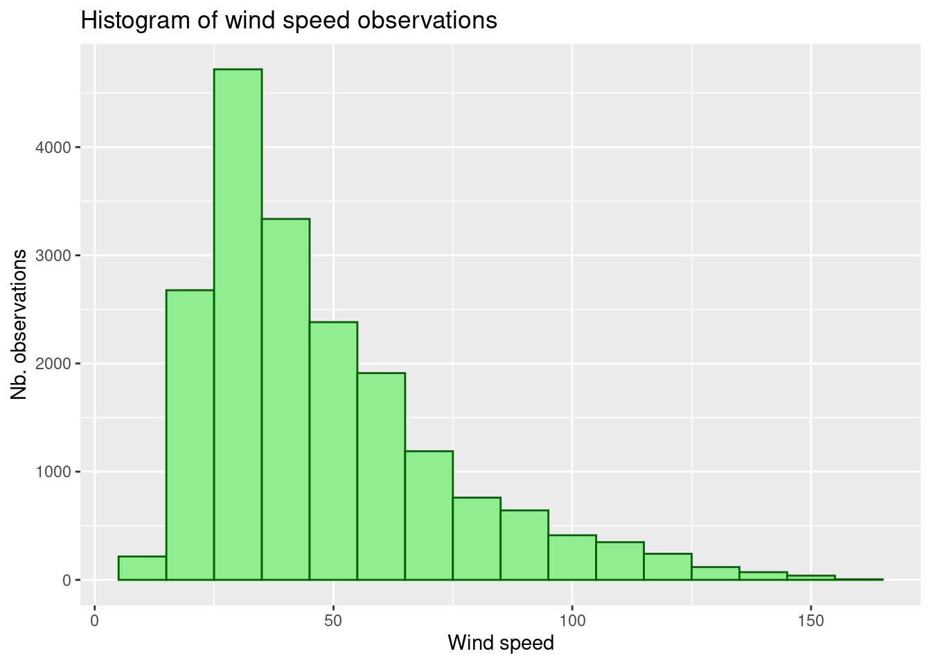
ggplot(storms, aes(x=wind))+labs(title="Histogram of wind speed observations",x="Wind speed", y="Nb. observations") +geom_histogram()
`stat_bin()` using `bins = 30`. Pick better value with `binwidth`.
Key Argument
To define the size of bins according to the x-axis use binwidth
ggplot(storms, aes(x=wind))+labs(title="Histogram of wind speed observations",x="Wind speed", y="Nb. observations") +geom_histogram(color ="darkgreen", fill ="lightgreen", binwidth=10)
geom_boxplot() & geom_violin()
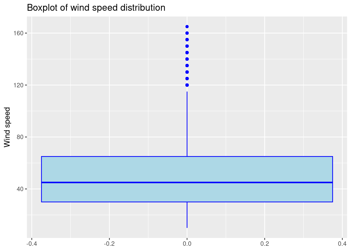
#### Use geom_boxplot() to create a boxplot
ggplot(storms, aes(y=wind)) +labs(title="Boxplot of wind speed distribution", y="Wind speed")+geom_boxplot(fill="lightblue", color="blue")
By default the plot is centered on the x-axis.
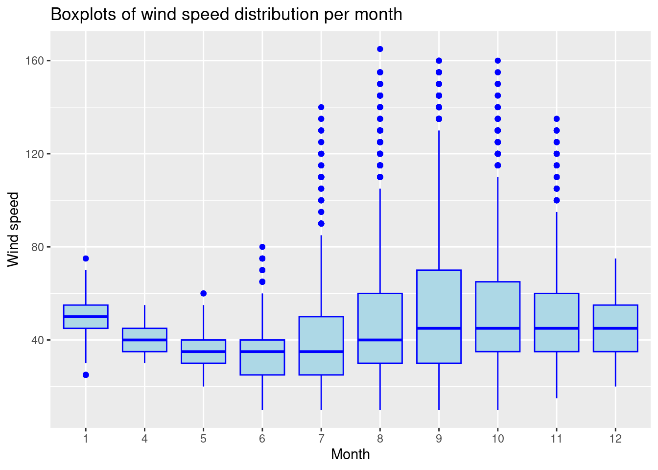
To show the distribution within different groups, in this example within each month:
ggplot(storms, aes(x=as.factor(month), y=wind)) +labs(title="Boxplots of wind speed distribution per month",x="Month", y="Wind speed")+geom_boxplot(fill="lightblue", color="blue")
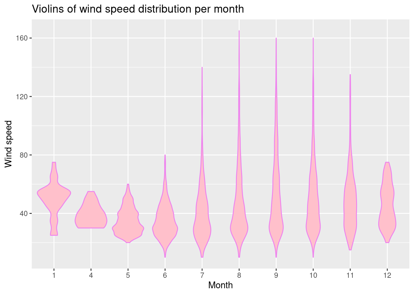
Use geom_violin() to create a violin plot
ggplot(storms, aes(x=as.factor(month), y=wind)) +labs(title="Violins of wind speed distribution per month", x="Month", y="Wind speed")+geom_violin(fill="pink", color="violet")
Presentation tips
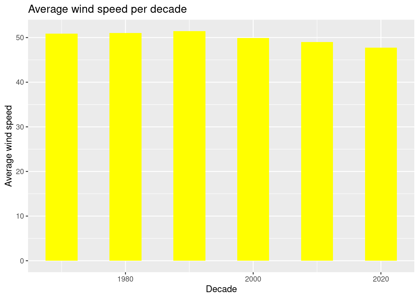
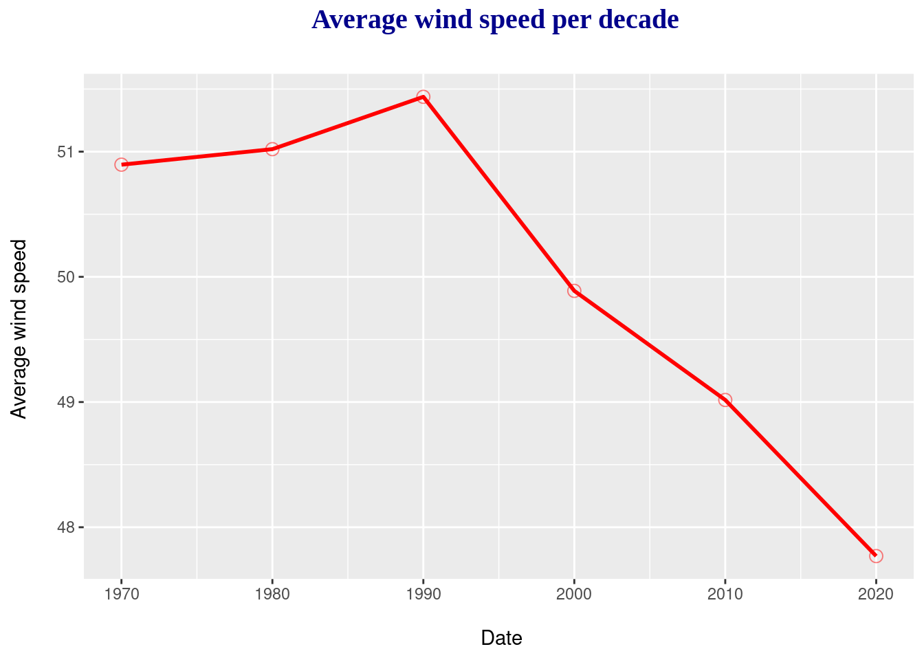
Theme customization with theme()
You can customize the prensentation of your graphics with theme(). We present here example for the plot title customization with the plot.title argument.
To bold the text use face `
To change the font size use size
To change the color use color
To adjust the position use hjust
** hjust =0.5 to center the title; 0 to put the title to the left, and 1 to put the title to the right.
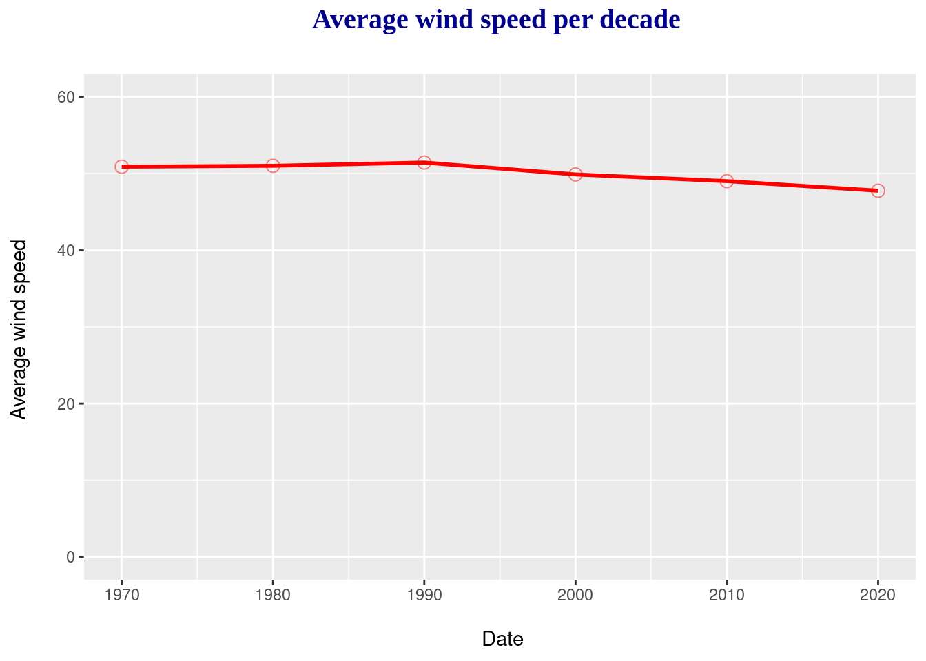
coord_cartesian() controls the extent of the graph axes. It allows you to explicitly define the limits of the x and y axes of the graph (useful for zooming in or out on a specific part of the graph, while keeping the original data!)
In this example, coord_cartesian(y=c(0,60)) allows to restrict the y-axis to the range from 0 to 60.
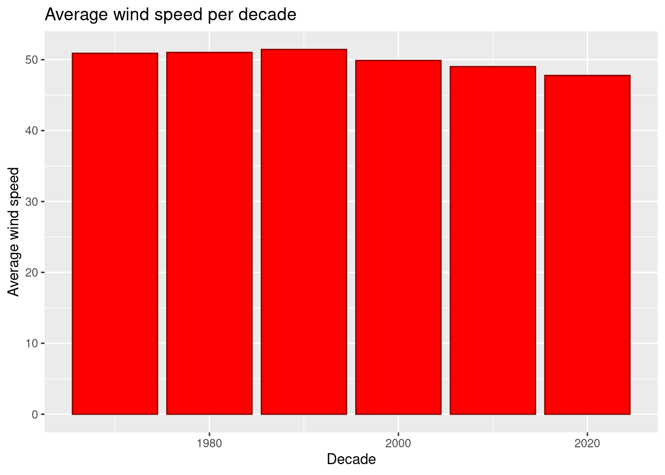
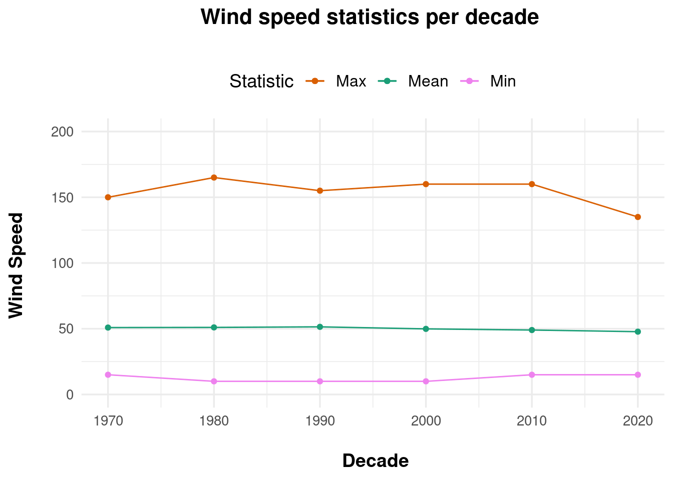
scale_color_manual()
The scale_color_manual() function is used to specify the colours associated with different values or levels of an aesthetic variable in a plot. With the name argument, you specify the title of the color legend. With the values arguments, you specify the colours associated with each value of the selected variable.
NB : scale_fill_manual() functions exactely the same.
theme(legend.X()) As for the title of the graphic, you can use theme.() function with legend.X, to put in bold, to change the size, the color, the position,… of the legend (its title, and its text).
ggarrange()
With the ggarrange() function you can organize your plots : their size, their marges, etc. For example, you can create graphics mosaics, which display several graphs side by side in a single figure.
First, ensure ggpubr is installed : install.packages('ggpubr')
library("ggpubr") #Load the library
You can personalize a theme for displaying the plots in the same way, by creating a function theme() with the options you want.
theme_custom <-function(...) {theme(plot.title =element_text(face ="bold", color="black", hjust =0.5), title =element_text(size=10))}
With title you change the plot title and the x-axis and y-axis. With plot.title you change only the title of your plot.
Choose your plots and store them as objects to use ggarrange()